An interesting paper about the artistry in a building of multi-factor portfolios:

Authors: Israel, Jiang, Ross

Title: Craftsmanship Alpha: An Application to Style Investing

Link: https://papers.ssrn.com/sol3/papers.cfm?abstract_id=3034472

Abstract:

Successful investing requires translating sound investment concepts into actual trading strategies. We study many of the implementation details that portfolio managers need to pay attention to; such choices range from portfolio construction to execution. While these kinds of decisions apply to any type of investment strategy, they are particularly important in the context of style investing. Consider two managers who both intend to capture the value factor in a long/short context: each manager might make a number of decisions, many of which can lead to meaningfully different outcomes. These choices can often explain why one value manager outperforms another. Ultimately, what may seem like inconsequential design decisions can actually matter a lot for style portfolios. In fact, the skillful targeting and capturing of style premia may constitute a form of alpha on its own — one we refer to as “craftsmanship alpha.”

Notable quotations from the academic research paper:

"Style premia are a set of systematic sources of returns that are well researched and have been shown to deliver longrun returns that are uncorrelated with traditional assets. Styles have been most widely studied in U.S. equity markets, but have been shown to work consistently across markets, across geographies, and over time. There are variations in the types of style portfolios, but also — importantly — in how different managers choose to build those portfolios. While practitioners might define styles with similar “labels,” actual portfolios can differ significantly from one another.

Our paper focuses on the craftsmanship required to build effective style portfolios. That is, the kind of decisions that happen after we have already agreed on the type of style portfolio that we want to build.

We start with a brief discussion of the types of style portfolios an investor may choose; we then go into more detail on design decisions related to building style portfolios; and finally, we address other considerations for style investing, such as trading and risk management. We will share our thoughts on a number of enhancements that can be made without deviating from the main thesis . While many of these enhancements reflect our opinions on better ways to build portfolios, the main point is that these choices need to be made consciously. Certain design choices may improve the risk/return characteristics of the overall portfolio, by enhancing returns, reducing risk, or a combination of both. We call the sources of alpha that involve implementation choices “craftsmanship alpha.”

Topics:

1. What Kind of Style Portfolio?
2. How to Build Style Portfolios?
  2.1. Smarter Style Measures
  2.2. Multiple Style Measures
  2.3. Stock Selection and Weighting Schemes
  2.4. Unintended Risks
  2.5. Volatility Targeting
  2.6. Integrating Styles in a Multi-Style Portfolio
  2.7. Strategic or Tactical
3. How To Execute Style Portfolios?
   3.1. Portfolio Implementation
   3.2. Cost-Effective Execution
   3.3. Risk Management
4. Conclusion
"

Are you looking for more strategies to read about? Check http://quantpedia.com/Screener

Do you want to see performance of trading systems we described? Check http://quantpedia.com/Chart/Performance

Do you want to know more about us? Check http://quantpedia.com/Home/About

If an investor wants to build multi-factor portfolio then he should look around and build a diversified global portfolio:

Authors: Binstock, Kose, Mazzoleni

Title: Diversification Strikes Again: Evidence from Global Equity Factors

Link: https://papers.ssrn.com/sol3/papers.cfm?abstract_id=3036423

Abstract:

The benefits of country diversification are well established. This article shows that the same benefits extend to equity factors, such as value, size, momentum, investment, and profitability. Specifically, country factor portfolios reflect both common variation, which we define as the global factor, and local variation. On average, a US investor could enjoy a 30% reduction in portfolio volatility by investing globally. We also document three other properties of equity factors. Like major asset classes, greater market integration is associated with greater factor co-movement, and factor portfolios of different countries tend to be more correlated during bear stock markets. However, unlike asset classes, the correlations of factor portfolios across countries have not been increasing over the last two decades, making global equity factors a particularly desirable addition to a portfolio.

Notable quotations from the academic research paper:

"In this paper, we bring the insights of geographic diversification to cross-sectional equities. We study the returns of long-short portfolios across developed countries based on six factors: market, value, size, momentum, investment, and profitability.

Our international equity factor analysis offers three novel insights.

First, by diversifying an equity strategy across developed markets, investors can significantly reduce the volatility of their factor portfolio. Even for a U.S. investor, who has access to a large domestic market, the volatility reduction across the factors is estimated up to 30%. Indeed, country factor portfolios reflect common variation, which we identify as the global factor, and “local” volatility. A global factor has a simple interpretation as the average world excess returns and tends to explain the individual strategies’ alpha. The local component reflects potentially uncompensated risk, which can be diversified away by simply investing across national markets.

Our second insight shows that factor strategies tend to be more correlated across more integrated countries. For instance, the correlation between the US and the UK stock markets is markedly higher than the correlation between the Japanese and UK markets. We find that these associations also extend to factor portfolios. Accordingly, the momentum strategies in the US and the UK markets are notably more correlated than the momentum strategies in the Japanese and UK markets.

Our last contribution highlights the time-series behavior of factor strategies during bear and bull markets, and across different decades. Previous studies show that return correlations tend to increase in bear markets. Consistent with these works, we document that country factor strategies tend to be more correlated during down-market periods, a phenomenon explained by rising global volatilities. Hence, even for equity factors, diversification fades when most needed. Yet, in contrast to the trends observed for major asset classes, we also document that these correlations have been relatively stable over different decades. This is good news for long-term investors who seek different sources of diversification.
"

Are you looking for more strategies to read about? Check http://quantpedia.com/Screener

Do you want to see performance of trading systems we described? Check http://quantpedia.com/Chart/Performance

Do you want to know more about us? Check http://quantpedia.com/Home/About

An interesting insight into problems associated with an attempts to implement machine learning in trading:

Authors: de Prado

Title: The 7 Reasons Most Machine Learning Funds Fail

Link: https://papers.ssrn.com/sol3/papers.cfm?abstract_id=3031282

Abstract:

The rate of failure in quantitative finance is high, and particularly so in financial machine learning. The few managers who succeed amass a large amount of assets, and deliver consistently exceptional performance to their investors. However, that is a rare outcome, for reasons that will become apparent in this presentation. Over the past two decades, I have seen many faces come and go, firms started and shut down. In my experience, there are 7 critical mistakes underlying most of those failures.

Notable quotations from the academic research paper:

"
• Over the past 20 years, I have seen many new faces arrive to the financial industry, only to leave shortly after.
• The rate of failure is particularly high in machine learning (ML).
• In my experience, the reasons boil down to 7 common errors:
1. The Sisyphus paradigm
2. Integer differentiation
3. Inefficient sampling
4. Wrong labeling
5. Weighting of non-IID samples
6. Cross-validation leakage
7. Backtest overfitting

Pitfall #1:
The complexities involved in developing a true investment strategy are overwhelming.  Even if the firm provides you with shared services in those areas, you are like a worker at a BMW factory who has been asked to build the entire car alone, by using all the workshops around you. It takes almost as much effort to produce one true investment strategy as to produce a hundred. Every successful quantitative firm I am aware of applies the meta-strategy paradigm. Your firm must set up a research factory where tasks of the assembly line are clearly divided into subtasks, where quality is independently measured and monitored for each subtask, where the role of each quant is to specialize in a particular subtask, to become the best there is at it, while having a holistic view of the entire process.

Pitfall #2:
In order to perform inferential analyses, researchers need to work with invariant processes, such as returns on prices (or changes in log-prices), changes in yield, changes in volatility. These operations make the series stationary, at the expense of removing all memory from the original series. Memory is the basis for the model’s predictive power. The dilemma is returns are stationary however memory-less; and prices have memory however they are non-stationary.

Pitfall #3:
Information does not arrive to the market at a constant entropy rate. Sampling data in chronological intervals means that the informational content of the individual observations is far from constant. A better approach is to sample observations as a subordinated process of the amount of information exchanged: Trade bars. Volume bars. Dollar bars. Volatility or runs bars. Order imbalance bars. Entropy bars.

Pitfall #4:
Virtually all ML papers in finance label observations using the fixed-time horizon method. There are several reasons to avoid such labeling approach: Time bars do not exhibit good statistical properties and the same threshold is applied regardless of the observed volatility. There are a couple of better alternatives, but even these improvements miss a key flaw of the fixed-time horizon method: the path followed by prices.

Pitfall #5:
Most non-financial ML researchers can assume that observations are drawn from IID processes. For example, you can obtain blood samples from a large number of patients, and measure their cholesterol. Of course, various underlying common factors will shift the mean and standard deviation of the cholesterol distribution, but the samples are still independent: There is one observation per subject. Suppose you take those blood samples, and someone in your laboratory spills blood from each tube to the following 9 tubes to their right. Now you need to determine the features predictive of high cholesterol (diet, exercise, age, etc.), without knowing for sure the cholesterol level of each patient. That is the equivalent challenge that we face in financial ML.
–Labels are decided by outcomes.
–Outcomes are decided over multiple observations.
–Because labels overlap in time, we cannot be certain about what observed features caused an effect.

Pitfall #6:
One reason k-fold CV fails in finance is because observations cannot be assumed to be drawn from an IID process. Leakage takes place when the training set contains information that also appears in the testing set. In the presence of irrelevant features, leakage leads to false discoveries. One way to reduce leakage is to purge from the training set all observations whose labels overlapped in time with those labels included in the testing set. I call this process purging.

Pitfall #7:
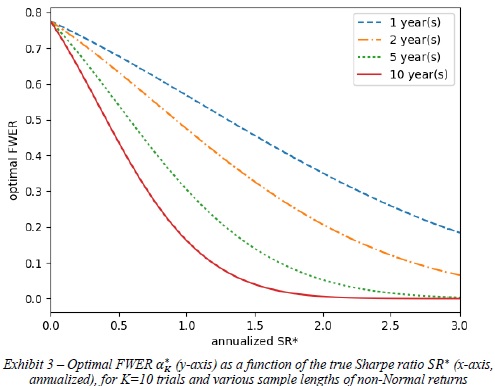
Backtest overfitting due to data dredging. Solution – use The Deflated Sharpe Ratio – it computes the probability that the Sharpe Ratio (SR) is statistically significant, after controlling for the inflationary effect of multiple trials, data dredging, non-normal returns and shorter sample lengths.
"

Are you looking for more strategies to read about? Check http://quantpedia.com/Screener

Do you want to see performance of trading systems we described? Check http://quantpedia.com/Chart/Performance

Do you want to know more about us? Check http://quantpedia.com/Home/About

How should investor weight commodity strategies in his portfolio? Is it better to use simple approach or some sophisticated weighting scheme?

Authors: Fernandez-Perez, Fuertes, Miffre

Title: Harvesting Commodity Styles: An Integrated Framework

Link: https://papers.ssrn.com/sol3/papers.cfm?abstract_id=3005347

Abstract:

This paper develops a portfolio allocation framework to study the benefits of style integration and to compare the effectiveness of alternative integration methods in commodity markets. The framework is flexible enough to be applicable to any asset class for either long-short, long- or short-only styles. We study the naïve equal-weighted integration and sophisticated integrations where the style exposures are sample-based by utility maximization, style rotation, volatility-timing, cross-sectional pricing or principal components analysis. Considering the “universe” of eleven long-short commodity styles, we document that the naïve integration enhances each of the individual styles in terms of their reward-to-risk tradeoff and crash risk profile. Sophisticated integrations do not challenge the naïve integration and the rationale is that, while also achieving multiple-style exposures, the equal-weighting approach circumvents estimation risk and perfect-foresight bias. The findings hold after trading costs, various reformulations of the sophisticated integrations, economic sub-period analyses and data snooping tests inter alia.

Notable quotations from the academic research paper:

"Recent studies have shown a lot of long-short style portfolios that are able to capture a premium – the most notably based on backwardation and contango, past performance, net short hedging and net long speculation, liquidity, open interest, inflation beta, dollar beta, value, volatility or skewness signals.

Instead of “putting all the eggs in one basket” (i.e., adopting one of the commodity investment styles mentioned above), the present paper is concerned with the idea of forming a long-short commodity portfolio that has exposure to many styles. Style integration has a strong economic appeal. By relying on a composite variable that aggregates information from various signals, the investor ought to predict more reliably the subsequent asset price changes. Relatedly, an integrated portfolio should benefit from signal diversification in the form of less volatile excess returns. For the above reasons, one may readily agree that style integration is a sensible approach that may improve performance relative to standalone style portfolios. This, however, begs the question: How do we integrate K styles at asset level (i.e., within a unique portfolio)? Specifically, how shall we decide the weights that the integrated portfolio allocates to each of the individual styles?

This paper makes three contributions to the style integration literature.

Our first contribution is to propose a simple, yet versatile, framework to conduct style integration. The proposed integration framework accommodates many variants pertaining to: i) the scoring scheme to rank the N assets according to each of the individual styles, and ii) the weighting scheme for the K individual styles (or the style exposures). The proposed framework is very flexible as it is applicable to long-only, short-only, as well as long-short investment styles, for any asset class. This contribution addresses an important goal of the paper which is to provide academics and practitioners with a well-structured way to blending multiple asset characteristics to improve
portfolio allocation. The framework proposed nests many integration methods. We formulate a naïve integration with time-constant, equal-weights for all styles (Equal-Weighted Integration; EWI), and various ‘sophisticated’ approaches with time-varying and heterogeneous style exposures determined by different criteria.

Our second contribution is to illustrate the flexibility of the integration framework by deploying the aforementioned strategies to the “universe” of styles in commodity futures markets in order to ascertain which integration method is most effective in practice. To our knowledge, no prior study (for any asset class) has conducted such a comparison of alternative style-integration approaches. Furthermore, there is a dearth of research on style integration in commodity futures markets. Our findings suggest that the naïve EWI portfolio stands out by generating very attractive reward-to-risk ratio profile (Sharpe, Sortino and Omega ratios) and lowest crash risk (downside volatility, 99% Value-at-Risk, and maximum drawdown) that is not challenged by the standalone portfolios nor the sophisticated integrated portfolios. The failure of the latter to outperform the EWI portfolio suggests that the benefits from allowing time-varying and heterogeneous exposures to the K styles are offset by estimation risk and perfect-foresight bias.

Our final contribution is to add to the debate as to whether holding the EWI portfolio is equivalent to investing a fraction 1/K of wealth into each of K independently-managed style portfolios. The EWI portfolio can be thought of as an “aggregate-then-invest portfolio” while the 1/K approach, also called portfolio mix, is an “invest-then-aggregate portfolio”. This debate has been confined to long-only equity styles thus far and we contribute to it by comparing theoretically and empirically the Sharpe ratio of both integration approaches for long-short commodity styles. We show that, even before transaction costs, the EWI portfolio achieves a higher reward per unit of risk than the portfolio mix because the latter randomly fails to fully invest the clients’ mandate.

"

Are you looking for more strategies to read about? Check http://quantpedia.com/Screener

Do you want to see performance of trading systems we described? Check http://quantpedia.com/Chart/Performance

Do you want to know more about us? Check http://quantpedia.com/Home/About

An important paper about correlation structure of anomalies:

Authors: Geertsema, Lu

Title: The Correlation Structure of Anomaly Strategies

Link: https://papers.ssrn.com/sol3/papers.cfm?abstract_id=3002797

Abstract:

We investigate the correlation structure of anomaly strategy returns. From an initial 434 anomalies, we select 116 anomalies that are significant in the mean and not highly correlated with other anomalies. Cluster analysis reveals 24 clusters and 29 singleton anomalies that can be grouped into 3 essentially uncorrelated blocks. Correlations between anomaly strategies exhibit some stability over time at both a pairwise and aggregate level. The exception is a correlation spike in 2001, possibly related to the aftermath of the dot-com crisis. In volatile markets correlations increase in magnitude while maintaining their sign. Short and long legs of the same anomaly are highly correlated but becomes largely uncorrelated once we use market excess returns, suggesting that the long and short legs of anomalies follow different dynamics once market-wide influences are compensated for. Correlations based on the residuals of benchmark models are substantially lower, with mean absolute correlation declining by up to half. The existence of 116 anomaly strategies that are not highly correlated echoes other findings in the literature that the return generating process for realised returns appears to be of a high dimension.

Notable quotations from the academic research paper:

"Our paper investigates the correlation structure of 434 anomaly strategies. To our knowledge we are the first to examine the correlation structure of anomaly strategies in detail on this scale. The importance of anomalies may be self-evident to researchers in the field. But what do we gain by investigating the correlation structure of anomalies? We advance three arguments to motivate our work.

First, we argue that the importance of an anomaly should depend on both its magnitude and its uniqueness relative to other anomalies. The magnitude of anomalies is both well studied and well reported. On the other hand, little is known about the uniqueness of a given anomaly relative to the rest. Most anomaly research conduct the usual time-series alpha tests on anomaly portfolios and may, in addition, control for a handful of other anomalies. At one extreme, a new anomaly might be so highly correlated with another anomaly as to essentially constitute the same effect, thus at best contributing a more nuanced understanding or interpretation of the original anomaly. At the other extreme, a new anomaly might be completely orthogonal to all known anomalies. Such an anomaly is clearly more valuable in furthering our understanding of the cross-section of realised returns. The correlation between anomalies allows us to quantify which anomalies are unique, which are related and which are essentially the same, thus imposing a measure of order on the factor zoo.

Second, understanding the correlation structure between anomalies (and its dynamics over time) may aid in uncovering the underlying sources of macro-economic risk that drives the compensation for-risk component of anomaly excess returns. Groups of anomalies that are consistently correlated may point towards common underlying factors, thus aiding in the construction of better expected return benchmark models.

Third, correlation, in combination with asset variance, completely determines the covariance matrix of asset returns. The return covariance matrix has played a central role in virtually all portfolio management since Markowitz.

We find that some anomalies are highly correlated with other anomalies, to the extent that it is very likely that they reflect the same latent effect. Once we restrict ourselves to the 151 anomalies that are significant in the mean, 36% percent of anomalies have an absolute pairwise correlation above 0.8 with some other anomaly. Despite this, 116 anomaly strategies remain even when we consolidate highly correlated anomalies (those correlated at 0.8 or above). A principal component analysis conducted on the 116 anomalies confirms the high-dimensionality of the dataset. A total of 60 principal components are needed to explain 90% of the variation in the 116 anomalies. Many finance researchers have a prior that there should be only a small number of independent sources of priced risk – and certainly not 60. An interpretation that avoids this tension is that much of the outperformance of anomaly strategies may be a combination of a) mispricing and b) data-mining.

We find clusters of anomalies that exhibit high within-cluster correlation. Between-cluster correlation ranges more widely from positive to negative. Together the pattern is one of intricate correlation structures that appear qualitatively different from either white noise or a simple linear factor data generating process. The anomalies grouped within clusters make sense, in that their similarity is evident from the way in which they are constructed. This enables us to assign to these 24 clusters tentative labels. In addition to the 24 labelled clusters, we also identify 29 “singletons” – single anomalies that can be thought of as clusters containing a single anomaly. At a higher level, we identify three “blocks” of anomalies. The pairwise correlations between anomalies in the same block are almost always positive, while the correlations between anomalies in different blocks are often negative.

Once we eliminate highly correlated anomalies and anomalies that are not significant in the mean, the average correlation between two distinct anomalies is 0.05. This very low average correlation has been cited as a reason why there is no need to control a new anomaly against every single existing anomaly. We find that the mean (across anomalies) of the maximum correlation relative to other anomalies is 0.68, dropping to 0.56 if highly correlated anomalies are consolidated. This suggests that at least some of the new anomalies proposed in the literature may not be as unique as previously thought.

There is evidence that the correlation structure of anomalies are state-dependent. In particular, we find that volatile months (those in the top quartile measured by daily market volatility) produce correlations with substantially higher magnitude but with the same sign as quiet months (those in the bottom quartile). In other words, positive correlations become more positive and negative correlations become more negative in volatile markets. This stands in contrast to the received wisdom that asset correlations tend toward one in volatile markets.

"

Are you looking for more strategies to read about? Check http://quantpedia.com/Screener

Do you want to see performance of trading systems we described? Check http://quantpedia.com/Chart/Performance

Do you want to know more about us? Check http://quantpedia.com/Home/About

A new financial research paper related to:

#75 – Federal Open Market Committee Meeting Effect in Stocks

Authors: Cocoma

Title: Explaining the Pre-Announcement Drift

Link: https://papers.ssrn.com/sol3/papers.cfm?abstract_id=3014299

Abstract:

I propose a theoretical explanation for the puzzling pre-announcement positive drift that has been empirically documented before scheduled Federal Open Market Committee (FOMC) meetings. I construct a general equilibrium model of disagreement (difference-of-opinion) where two groups of agents react differently to the information released at the announcement and to signals available between two announcement releases. In contrast to traditional asset pricing explanations, this model matches key empirical facts such as (1) the upward drift in prices just before the announcement, (2) lower (higher) risk, price volatility, before (after) the announcement occurs, and (3) high trading volume after the announcement, while trading volume is low before the announcement occurs.

Notable quotations from the academic research paper:

"It seems implausible that price increases in the aggregate equity market occur persistently and at scheduled points in time without any associated risk. Still, this was the description of the pre-announcement drift puzzle found in
Lucca and Moench (2015), henceforth LM. The authors documented a persistent upward drift in equity prices together with very low volatility before the scheduled announcements of the FOMC meetings. This paper seeks to provide a theoretical framework to explain how such a positive drift persist and species what kind of risk is embedded in it.Over the past decades, stocks in aggregate have experienced large positive excess returns in anticipation of scheduled FOMC announcements and, to a certain extent, in anticipation of scheduled corporate earnings announcements. I will refer to this phenomenon as the pre-announcement drift. I will claim that, while traditional asset pricing explanations would fail to match the empirical evidence, a model of disagreement based on Dumas et al. (2009), henceforth DKU, creates sentiment risk that matches the stylized facts documented empirically in the literature.

I present a general equilibrium model in which two groups of agents have differences-of-opinion about the content of an announcement. In this economy, there is a continuous stream of dividends being paid, but the rate of growth
of these dividends is unknown and not directly observable. All investors receive information from the current dividend and a signal they may choose to acquire about the unknown growth rate. Agents have different beliefs about the
correlation between their information sources, announcement and signal, and the unobserved rate of growth of dividends. This heterogeneity in the correlation makes the expectations of two groups of agents differ; I will henceforth
call the fluctuations in the beliefs of the two groups as changes in "sentiment". The single parameter in this model that sets it apart from traditional rational-expectations general equilibrium models is the non-zero correlation between the information sources and the unobserved rate of growth. In this model, agents will always have a source of difference-of-opinion because they disagree on a fixed parameter of the model. They, therefore, do not learn from each other's behavior nor from price but simply "agree to disagree".

The intuition of the model in this paper is the following: When an announcement about the unobserved growth rate of the economy occurs, there will be a discontinuous jump in disagreement. This happens because agents will have different interpretations of the information released at the announcement; they assume different correlations of the announcement release and the unknown growth rate. Over time, in the period between announcements, agents will in general remain at a certain level of disagreement, because at least one group of agents acquires a signal about the unobserved growth rate of the economy that the other group of agents does not acquire. Once the next announcement becomes imminent, it would be optimal for all agents to stop acquiring any signal because a new announcement will make all previous information stale. There will be an optimal point in time when the acquiring costs will outweigh the benefits from potentially using the information to be acquired. Therefore, agents will choose not to acquire information, which will bring agents to drastically reduce their disagreement level.

When agents stop acquiring signals, the reduction in disagreement leads to a reduction of sentiment risk that manifests as an increase in prices; this increase in prices will match the pre-announcement drift. Low volatility will be observed in the pre-announcement period, where there is low sentiment risk; and high volatility will be observed after the announcement, where there is an increase in sentiment risk. Finally, high trading volume will occur just after the announcement is released, since this is the point in time with the highest level of disagreement and it would be at its lower point just before the next announcement occurs."

Are you looking for more strategies to read about? Check http://quantpedia.com/Screener

Do you want to see performance of trading systems we described? Check http://quantpedia.com/Chart/Performance

Do you want to know more about us? Check http://quantpedia.com/Home/About