In-Sample vs. Out-Of-Sample Analysis of Trading Strategies
Science has been in a “replication crisis” for more than a decade. Researchers have discovered, over and over, that lots of findings in fields like psychology, sociology, medicine, and economics don’t hold up when other researchers try to replicate them. There are many interesting questions of philosophy of science, for example: Is the problem just that we test for “statistical significance” — the likelihood that similarly strong results could have occurred by chance — in a nuance-free way? Is it that null results (that is when a study finds no detectable effects) are ignored while positive ones make it into journals? Simply said: many published studies cannot be replicated.
But what does it mean to us, investors and traders? We, here at Quantpedia, try to present you academic research in a digestible form for the person that is not used to going rigorously through myriads of papers written in “academese” and often hard to understand true applicable meaning of it.
So, is there any “edge” in purely academic-developed trading strategies and investment approaches after publishing, or will they perish shortly after becoming public? After some time, we are about to revisit our own concept and test the out-of-sample decay. But this time, we have hard data – our regularly updated database of replicated quant strategies.
Introduction
When an anomaly is discovered and a strategy built around it is shared, it often leads to concerns that the anomaly might be arbitraged away and potentially turning unprofitable in investors’ portfolios. However, investment strategies typically remain profitable after publication, although there is a decrease in profitability. However, the returns do not instantly weaken; a significant part of the return remains even after the strategy becomes widely known. A study conducted by McLean and Pontiff found that portfolio returns were 26% lower out-of-sample and 58% lower during the five years post-publication, indicating that investors are aware of academic publications and learn about mispricing. However, the diminishing of returns happens gradually over time, and even after five years, a remarkable part of an anomaly’s return is preserved. The known anomaly often transforms into a ‘smart beta factor’ and can still be profitably used within a diversified portfolio. It’s also noted that the publication process of academic papers can take one or two years, and during this time, practitioners can extract ideas from working papers to gain an advantage.
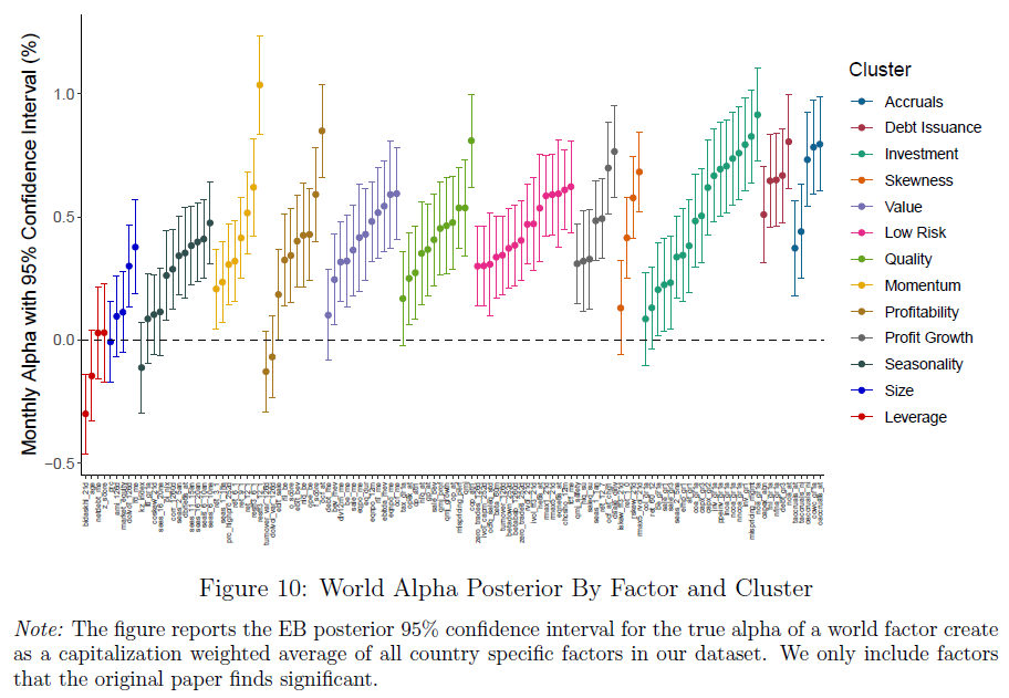
A recent paper by Jensen, Kelly & Pedersen: Is There a Replication Crisis in Finance? also discusses the replication of trading strategies described in academic research. The researchers found that over 80% of US equity factors remained significant even after making adjustments for consistent and more implementable factor construction while still preserving the original signal. In addition, the same quality and quantity of behavior were observed across 153 factors in 93 countries, suggesting a high degree of external validity in factor research. That’s really not a bad result …
Not too much disturbing are also findings from Heiko Jacobs and Sebastian Muller in their Anomalies across the globe: Once public, no longer existent? Motivated by McLean and Pontiff (2016) (which we will mention later), they studied the pre- and post-publication return predictability of 231 cross-sectional anomalies in 39 stock markets. Based on more than two million anomaly country months, their result is that the United States is the only country with a reliable post-publication decline in long/short returns. This might provide invaluable insights into the modeling of the “longevity” of strategies performed on these markets and “life expectancy” until strategy/anomaly “dies.”
The last research paper that we would like to mention is that of Falck, Rej, and Thesmar (2021), which examines the hypothesis of ex-ante characteristics empirically predicting the out-of-sample (they define out-of-sample as the post-publication period) drop in risk-adjusted performance of published stock anomalies. Their final conclusion is that every year, the Sharpe decay of newly-published factors increases by around 5% (which is not so much).
Data & Methodology
We have collected all data about strategies from our backtests (the ones you see in the end section of most of the Quantpedia Strategies found in our Screener) that were done in QuantConnect. Next, we diligently get information about when the data from the source papers end (end of data set testing period in the source academic paper). This bases the intersection between out-of-sample and in-sample for our backtests. Next, we divide these data into those two sets and compare and analyze them.
Let’s now show you our selected methodology for this experimental validation of our backtests on one example:
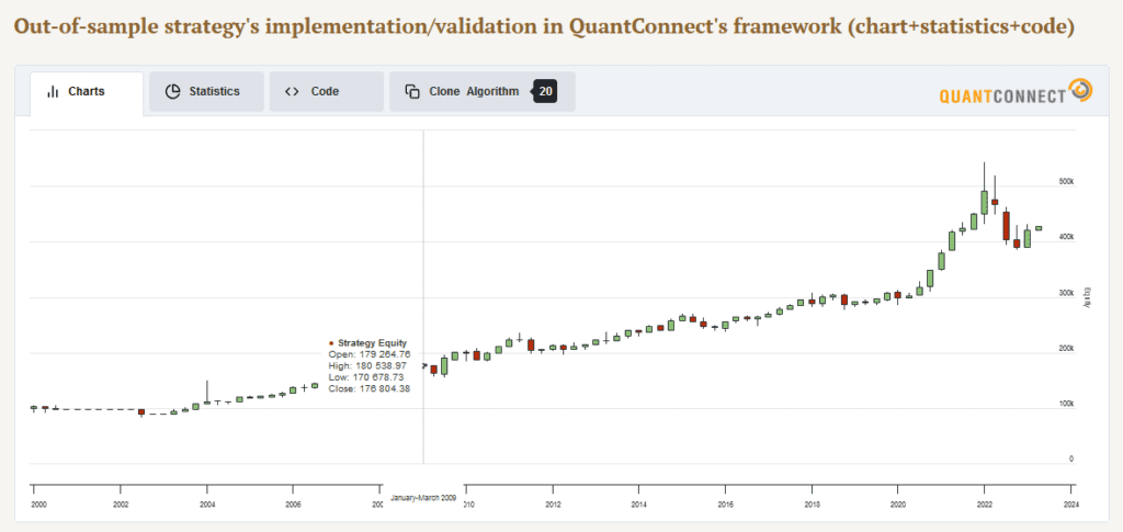
Let’s use our first-ever encyclopedic entry, the evergreen Asset Class Trend-Following strategy, based on Mebane Faber’s paper A Quantitative Approach to Tactical Asset Allocation. End of the backtesting period from paper sets point of intercept between datasets (the year after the hyphen) (on picture highlighted with green):

And this is being that year shown in QUANTCONNECT backtest. Up until the last day of 2008, we consider it in-sample backtest results, onwards from the first trading day of 2009 out-of-sample backtest results.
From all 868 strategies at the moment of analysis (at the beginning of May 2023), we have in-house backtested 671 out of them. Out of those, 417 were maintained and updated on a monthly basis, and those were therefore included in the analysis (and they can also be further used in Quantpedia Pro‘s Portfolio Manager and analytical tools). Further, 62 of them were excluded; we did not have data to get back into the period ending from the paper (we started backtesting from a date later than the end date of the data sample indicated in the paper). This concludes the data preprocessing part. So, we are left with 355 strategies for further analysis.
The main analyzed core interest is the Sharpe Ratio, which we conclude is the most suitable measure to compare in- vs. out-of-sample results in our data sample. Our database covers all main asset classes (equities, bonds, commodities, cryptos). Therefore, it would be meaningless to draw conclusions from annualized return measures when our data sample contains highly volatile crypto strategies and, at the same time, low volatile fixed-income strategies. The Sharpe ratio measure is great in our case because we scale annualized returns by yearly volatility, which helps to analyze risk-adjusted returns.
So, now we have both:
- in-sample dataset (usually
StartDatefrom QP until the end of Backtest period from source paper), - out-of-sample dataset (end of Backtest period from source paper until the end of QP backtest; in case of one-time-off code with limited data, is fixed, in case of recurring and updating code, always dynamic and adjusted to current month);
We calculated CAR p.a. and Volatility p.a., which division gave us Sharpe Ratios for in-sample and out-of-sample for each included strategy.
Results and their Interpretation
Now, let’s move on. As a measure of average, we have chosen the arithmetic mean. The median is the value separating the higher half from the lower half of a data sample and is not skewed by a small proportion of extremely large or small values, providing a better representation of the center. It is the main reason why we include it in our analysis too. The following table depicts the average and median Sharpe Ratios among the in- and out-of-sample data:
| Sharpe Ratio (of) |
average | median |
| in-sample results | 1.574 | 1.180 |
| out-of-sample results | 1.049 | 0.662 |
| Δ (in-out) | -0.525 | -0.518 |
| Δ% (in/out) | -33.37% | -43.90% |
As per Tab. 1, Sharpe Ratio for out-of-sample results is worse and deteriorated by 33% (on average) or 44% (median strategy). These results are totally in line and consistent with findings in the previously mentioned research papers and previous blog post we wrote about this topic.
Following is the figure depicting the distribution (histogram) of Sharpe Ratios both in- and out-of-sample:
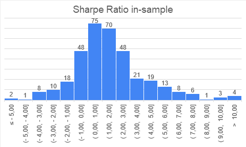

As we can see, the distribution of results follows “quasi-normal distribution”, where you can mainly expect your strategy to have a Sharpe ratio in interval (-1, 3). And it is both for out-of-sample and in-sample results. In-sample results are, of-course, faring a bit better.
Another interesting observation is that both in-sample and out-of-sample results seem to be skewed positively – fat tail on the right side (but the out-of-sample histogram right tail is a little less thick). This is a very interesting finding and speaks in favor of stringent risk management if we employ a portfolio of multiple strategies. It seems strategies seem to deteriorate an out-of-sample, but we have some really strong positive outliers; therefore, it makes sense to cut the risk budget to strategies that do not perform well out-of-sample and let profit runs in those that profit well. Those results may give some validity to the idea of Factor Momentum – it may be a good idea to increase weight for strategies that recently performed well.
But let’s move on. This is the picture showing how all included strategies behaved during the 10-year window, the last 5 years of in-sample, and the first 5 years in out-of-sample:
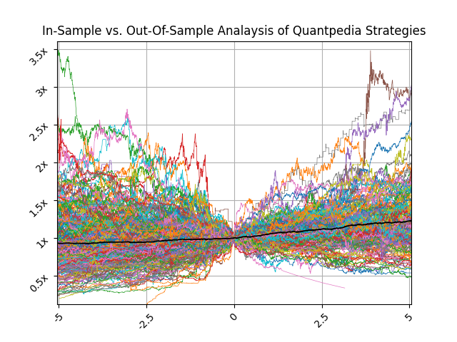
On X-axis, we have an in-sample period (-5 to 0), year zero is the threshold year, and from year 0 to 5 is the performance in the out-of-sample period. Y-axis shows an appreciation of 1 USD during the previously mentioned time. All strategies in year 0 start at 1 USD. The black line depicts the (simple arithmetic) average multiplier of returns when we mix all strategies in an equally-weighted portfolio. Our point here is to show that performed strategies have positive expectancy, but dispersion in performance (in- and also out-of-sample) is really significant.
Assuming we build a portfolio incorporating all backtested strategies weighted equally (black line), we also calculated what would be signal loss in performance after publication. Following our indicated approach, if you start using each strategy on the date when it ends being backtested by paper and weight your portfolio equally, we found that the out-of-sample portfolio would on average yield approximately 4/5 of in sample performance. Once again, individual performance decay among strategies varies a lot.
The performance decay in the portfolio approach is lower than performance decay in individual strategies. The reason for that is the low correlation among strategies (in- and also out-of-sample).
Conclusion
Undoubtedly, Sharpe Ratios worsen during a lifetime after forming various trading strategies based on beforehand not-know market anomalies. According to our analysis, it is reasonable to expect a Sharpe ratio degradation by 1/3 or by 1/2 against the in-sample period. This should not be, by any means, discouraging, but rather a positive finding that one should embrace and prepare to account for less pleasant sides of investing and trading, considering reported and expected returns and unexpected deviations from them.
Our results are in line with the current academic consensus. As in our previously mentioned blog post from 2020, McLean and Pontiff (2016) find that portfolio returns performing various trading strategies based on a statistically significant sample of different variables and factors covering the representable number of anomalies in total are 26% lower out-of-sample and 58% lower post-publication, which is not far away from our numbers.
What could be the partial solution for the performance decay? Preliminary findings suggest that factor momentum could be the right answer. Fat-tailed financial distributions are known to be good targets to exploit by momentum/trend-following rules. So momentum/trend overlay on a portfolio of strategies can be a good idea. Alternatively, other price-based factor overlays (low volatility, MIX, MAX, etc.) may also be considered, as we reviewed in our series of blog posts in which we investigated Social Trading Multi-Strategy (1, 2, 3, and 4).
Author:
Cyril Dujava, Quant Analyst, Quantpedia
Are you looking for more strategies to read about? Sign up for our newsletter or visit our Blog or Screener.
Do you want to learn more about Quantpedia Premium service? Check how Quantpedia works, our mission and Premium pricing offer.
Do you want to learn more about Quantpedia Pro service? Check its description, watch videos, review reporting capabilities and visit our pricing offer.
Are you looking for historical data or backtesting platforms? Check our list of Algo Trading Discounts.
Would you like free access to our services? Then, open an account with Lightspeed and enjoy one year of Quantpedia Premium at no cost.
Or follow us on:
Facebook Group, Facebook Page, Twitter, Linkedin, Medium or Youtube
Share onLinkedInTwitterFacebookRefer to a friend