Multi Strategy Management for Your Portfolio
If you follow Quantpedia’s blogs, you probably know that Quantpedia PRO already contains multiple risk management and portfolio construction tools for your quantitative investment strategies. For example, Crisis Hedge can find you suitable investment hedges for negative months and for bear markets. The Correlation Analysis report, on the other hand, reviews your model portfolio’s correlation structure. Alternatively, Value at Risk (VaR report) will help you understand what level of risk you can expect from your portfolio during a crisis. The newest Quantpedia PRO tool (available in a few days) will analyze something completely different, though – how to manage multi-strategy portfolios.
This report focuses on simple multi-strategy overlays based on trend-following and mean-reversion. In other words, we look into whether it is better to increase weights of the well-performing strategies and decrease those of bad-performing ones or if the opposite strategy is more profitable.
You can easily apply these multi-strategy overlays to various types of underlying – ETFs, systematic strategies, multi-asset portfolios, or multi-strategy portfolios. This article again serves as a primer for the new report’s methodology.
How to manage a Multi Strategy portfolio
There are countless debates on the topic of managing multi-strategy portfolios. Quantpedia has already published several articles addressing this problem. Risk Parity Asset Allocation examines and explains three methodologies of risk allocation which ensure an equal level of risk among assets in a portfolio. Another article called “The Active vs Passive: Smart Factors, Market Portfolio or Both?” discusses when and whether it is better to invest in the market itself or pick specific factors. Additionally, several Quantpedia PRO tools, such as Volatility Targeting or Markowitz Model, also look into the problem. The mentioned tools focus mainly on the risk aspect of underlying assets. That’s one of the reasons why we will today mostly focus on return.
Today, in our Multi-Strategy Management report, we apply multiple trend-following and contrarian strategy overlays with signals based on the performance of the underlying strategies. We analyze various time horizons from short-term (3-months), mid-term (12-moths) to long-term (24-months). Moreover, we apply these overlays to the original unadjusted strategies and also to the volatility-adjusted strategies.
Why do we look also at volatility adjusted strategies? Volatility adjustment is practical when portfolio contains assets or strategies with very different volatilities. In such a case, it is helpful to equalize the volatility contributions of the underlying strategies. After the volatility adjustment, all of the strategies should have the same chance to appear among the best/worst performing strategies. If we use the strategies with unadjusted volatility contributions, some strategies might have a higher chance of being at the top/ bottom, just because of their high volatility and not the actual performance.
Cross Asset Strategy use case
Data
We analyzed ten strategies from the Quantpedia screener. To create a diversified portfolio, we picked strategies covering various markets: stocks, commodities, currencies, multi-asset.
Our strategies include:
- Asset Class Momentum Rotational System
- FX Carry Trade
- Low Volatility Factor Effect in Stocks
- Currency Momentum Factor
- Pairs Trading with Stocks
- Momentum Effect in Commodities
- Term Structure Effect in Commodities
- FED Model
- Short Term Reversal with Futures
- Betting Against Beta Factor in Stocks
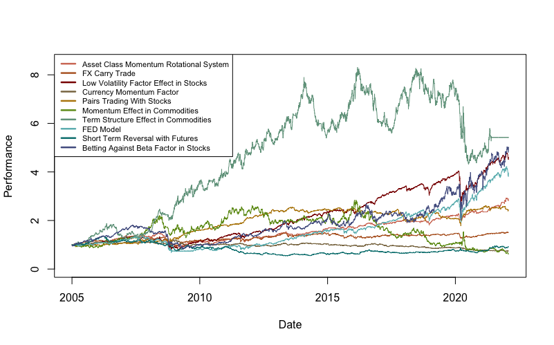
We may observe that this is a nice jungle of pretty different systematic strategies. Not only they differ in terms of underlying assets or volatilities, some of them perform well and some of them perform badly. Now what would happen if we applied systematic multi strategy management rules on top of the existing strategies? Let’s find out in the following sections.

Methodology
We analyze two different approaches – the cross sectional and the time series approach. In the cross-sectional approach, we apply cross-sectional momentum and cross-sectional reversal to the source multi-strategy portfolio. By “cross-section” we mean our 10 individual strategies. In the time series approach, we apply moving average overlays to each strategy individually, regardless of the performance of other strategies.
We also analyze the time-horizon sensitivity of these strategy overlays. For example, is it better to use the short-term, medium-term, or the long-term overlays?
Cross sectional management
More specifically, in the first approach, once a month we calculate the 3-month performance of the underlying strategies and sort them from the highest 3-month return to the lowest.
Then we create three types of equally weighted portfolios. The first type goes long the top 1 (/top 2 /top 3 /top4 /top5) underlying strategies. The second type goes long the bottom 1 (/bottom 2 /bottom 3 /bottom4 /bottom5) underlying strategies. The third type goes long the top 1/2/3/4/5 strategies, and shorts the bottom 1/2/3/4/5 underlying strategies.
Lastly, we repeat the same process outlined above to create the same three portfolios for mid-term (12-month) performance and long-term (24-month) performance.
Time series management
The second approach is based on moving averages. Every month we calculate the 3-month moving average of each underlying strategy and determine whether the strategy is above or below its MA. Then we create three portfolios. All of them are equally-weighted, with a maximal weight of 25% (the rest stays in cash).
The first portfolio goes long all the strategies that are above their respective MAs. The second portfolio goes long all the strategies below their respective MAs. And the last portfolio goes long the strategies that are above their 3-month MA and shorts the strategies below their respective 3-month MAs. Additionally, we created same portfolios for mid-term (12-month) MA and long-term (24-month) MA.
We start with original, volatility-unadjusted strategies. In the last section, we analyze the same strategy overlays also for volatility adjusted strategies.
Results: cross-sectional
Let’s now look at the results of all of the above-mentioned portfolios. We will start with cross-sectional strategies. The first figure shows the portfolios that go long the top 1 (/top 2 /top 3 /top4 /top5) underlying strategies based on a 3-month performance and compares them against the benchmark, set as an equally-weighted portfolio of all 10 strategies (black line).


The five portfolios outperformed the benchmark until the Corona crisis of 2020. After the crisis, only two portfolios performed better than the benchmark, the portfolio consisting of top 3 strategies and top 5 strategies. Results don’t seem to be much better than the benchmark.
The second figure illustrates the portfolios that go long the bottom 1 (/bottom 2 /bottom 3 /bottom4 /bottom5) strategies based on 3-month performance and the benchmark. We may observe, that this time the situation is different. The three most concentrated reversal overlays (picking 1/2/3 strategies) outperform the benchmark notably, although with higher volatility. It seems, on this short horizon, the cross-sectional reversal works better.


Lastly, we present the long-short portfolios based on top minus bottom 3-month performance of strategies. Unsurprisingly, given the results above, neither of these long-short portfolios outperformed the benchmark.


Similarly, the following figures show the portfolios based on 12-month and 24-month performance horizons.
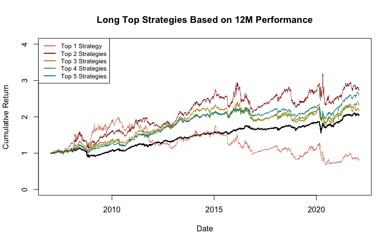
With the 12M horizon, momentum seems to be better than reversal, although outperformance isn’t stable, nor huge.


Long-short overlays on 1-year horizon don’t really seem to be different from a random walk.


On the longest horizon under scrutiny, momentum strategy overlays seem to be dominant. We can finally conclude, that momentum overlay seems to be performing well on this 2-year long horizon.


Results: time series
Secondly, let’s now look at time-series strategies. In the section below, we analyze the results of the portfolios created based on the Moving Averages of the underlying strategies.
The figure below shows the cumulative performance of the portfolio that goes long all of the strategies above (/below) their respective 3-month MA. Additionally, we also depict the portfolio that goes long the strategies above their respective MA and shorts the strategies below their respective MA, and the equal weight benchmark.

As we can see, neither of the portfolios outperformed the benchmark. However, when we applied 12-month MA, the portfolio that longs the strategies above their respective MA slightly outperforms the benchmark equally-weighted portfolio.

Lastly, looking at the portfolios’ performances based on 24-month MA, we can say that the portfolio that goes long the strategies above their respective MA significantly outperformed the benchmark.


Cross Asset Strategies with Volatility Targeting
Lastly, we repeated the whole process with volatility-targeted strategies. We decided to apply the volatility adjustment because of significant differences between volatilities of our underlying strategies. Equalizing the volatility contributions allows for the same chances for all strategies to appear in the top/bottom portfolio based on their performance.
The first figure shows the volatility targeted strategies, with targeted volatility of 10% p.a., and the benchmark, equally-weighted portfolio of all 10 volatility targeted strategies.


And now, let’s look at the same portfolios as in the previous section created from the volatility adjusted strategies. For the sake of brevity, we present only the equity curve charts and only for the cross-sectional strategies and skip the long-short portfolios (except 24-month horizon). That being said, we depict cross-sectional management based on 3-month (/12-month /24-month) performance compared with the benchmark.


Conclusion
We believe that systematic multi-strategy overlays provide valuable insight into multi-strategy portfolio management. We analyzed various strategy overlays based on trend-following and mean reversion on different time horizons.
For our specific set of strategies, the most profitable approach seemed to be the long-term trend-following. The results also indicate a presence of a short-term reversal in the underlying strategies. This, however, is not the case for mid or long-term periods. Both portfolios based on 12- and 24-month performances performed better when going long the strategies with the highest performances, indicating a long-term trend.
The subsequent section analyzed overlays based on moving averages. Once again, the portfolio based on long-term MA delivered the best results. Specifically, the portfolio which went long the strategies above their respective 24-month MAs.
Last but not least, we applied volatility adjustment to our underlying strategies. After the adjustment, we’ve ran through all the strategy overlays again and analyzed the results. Volatility adjustment may be helpful in case of significantly different volatilities of the underlying assets.
When to overweight and when to underweight your strategies is a very tough question, that every portfolio manager has to ask themselves regularly. In this article we presented one possible way of answering this question. We hope we inspired you at least a bit and will strive to do so also in our future articles.
Author:
Daniela Hanicova, Quant Analyst, Quantpedia
Do you want to learn more about Quantpedia Premium service? Check how Quantpedia works, our mission and Premium pricing offer.
Do you want to learn more about Quantpedia Pro service? Check its description, watch videos, review reporting capabilities and visit our pricing offer.
Or follow us on:
Facebook Group, Facebook Page, Twitter, Linkedin, Medium or Youtube
Share onLinkedInTwitterFacebookRefer to a friend