Shorting Leveraged ETFs: The Role of Borrowing Costs and Rebalancing in Volatility-Decay Strategies

Leveraged ETFs provide amplified exposure to an underlying index, but their daily reset mechanism creates volatility drag, which can substantially reduce their long-term value. This raises the possibility of exploiting the effect by simultaneously shorting leveraged ETFs with opposite exposures. We examine a 50/50 short portfolio of TQQQ and SQQQ, which provides approximately neutral exposure to the Nasdaq-100 while seeking to capture volatility decay. We analyze the strategy explicitly incorporate borrowing costs. We further investigate daily and weekly rebalancing, execution timing, and tranche-based rebalancing over five-, ten-, and twenty-day horizons. The results show that borrowing costs materially reduce the apparent profitability of the strategy. Moreover, after costs, returns are concentrated in a small number of high-volatility periods, while the strategy is largely neutral during ordinary market conditions. The findings demonstrate that ignoring short-selling costs and implementation details can substantially overstate the attractiveness and robustness of volatility-decay strategies.

Introduction

Leveraged exchange-traded funds (ETFs) have become increasingly popular as instruments for obtaining amplified exposure to financial markets. Among the most actively traded examples are the ProShares UltraPro QQQ (TQQQ) and ProShares UltraPro Short QQQ (SQQQ), which target three times the daily return and three times the inverse daily return of the Nasdaq-100 Index, respectively.

Because these ETFs reset their leverage every trading day, their long-term performance depends on the path of the underlying index rather than simply on its cumulative return. This creates the well-known volatility drag effect. For example, suppose an index rises by 5% on one day and falls by approximately 4.76% on the next day, leaving it almost exactly at its initial level. A 3× leveraged ETF would instead experience approximately a +15% return followed by a −14,28% return, resulting in a value of about 98.58% of its initial value. The underlying index has therefore returned approximately 0%, while the leveraged product has lost more than 1.4%.

This effect becomes stronger as the frequency and magnitude of fluctuations increase. For investors holding leveraged ETFs, volatility drag is therefore an important source of performance deterioration. For an investor taking the opposite position, however, the same mechanism may represent an opportunity.

This motivates a simple question: Can volatility drag be exploited by shorting both sides of a leveraged ETF pair?

In the case of TQQQ and SQQQ, the two products have opposite exposure to the same underlying index. Shorting them in equal proportions therefore largely cancels their first-order directional exposure. At the same time, both positions may benefit from the loss of value caused by daily compounding. The resulting portfolio can thus be viewed as an approximately directionally neutral strategy whose intended source of return is volatility decay.

Similar ideas have already been investigated in previous work. In particular, the Quantpedia strategy database includes approaches exploiting leveraged-ETF decay and arbitrage, including Arbitraging Levered ETFs [Quantpedia¹; other article²] and Volatility Decay and Arbitrage in Leveraged ETFs [Quantpedia³; other article⁴]. These strategies report relatively consistent historical returns. More recently, Volatility Decay Capturing⁵ described the strategy examined in this paper, although without incorporating borrowing costs and other practical considerations. The authors themselves point out that the reported results may therefore be unrealistic.

A key issue, however, is that the cost of borrowing the securities required for the short positions is not incorporated into these benchmark strategies. The reported returns may therefore represent a theoretical upper bound rather than a realistic estimate of what could have been earned in practice.

We consequently examine the effect of borrowing costs on the TQQQ–SQQQ strategy. We also consider another practical issue: maintaining the 50/50 allocation requires periodic rebalancing. The frequency and timing of this rebalancing may themselves have a substantial impact on performance.

Our analysis therefore addresses three main questions. First, how much of the apparent return survives after borrowing costs are included? Second, how sensitive is the strategy to the frequency, day, and timing of rebalancing? Third, can tranche-based rebalancing make the strategy more robust to the choice of a particular execution date?

Data

We used live data on QuantConnect for TQQQ and SQQQ over the period from July 13, 2015 to August 8, 2026. TQQQ targets three times the daily performance of the Nasdaq-100 Index, while SQQQ targets three times its inverse performance.

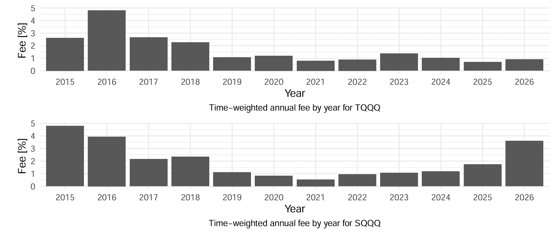
Over the same period, we also use borrowing-cost data for both securities. This allows us to compare the theoretical performance of the strategy with a cost-adjusted version that explicitly accounts for the cost of maintaining the required short positions.

Methodology

The basic strategy consists of a simultaneous short position in TQQQ and SQQQ:

weigth of TQQQ: -50%, weigth of SQQQ: -50%

Since the two ETFs provide opposite daily exposure to the Nasdaq-100, their directional effects largely offset each other. The portfolio is therefore approximately directionally neutral, while its return is driven primarily by the difference between the cumulative performance of the two daily-reset leveraged products. The strategy is rebalanced to maintain the intended 50/50 allocation.

The benchmark follows the same portfolio construction and rebalancing rules but assumes zero borrowing costs. It therefore represents the theoretical return of the strategy before accounting for the cost of shorting TQQQ and SQQQ.

The cost-adjusted strategy incorporates the observed borrowing costs of both securities. The difference between the two versions measures the impact of short-selling costs on the apparent volatility-decay return. This distinction is central to the analysis. A strategy can generate a positive return from volatility decay while still failing to generate an attractive net return once the cost of borrowing the underlying securities is considered.

Rebalancing

The 50/50 allocation of the two short positions cannot be maintained passively. As TQQQ and SQQQ move in opposite directions, their relative weights change, making periodic rebalancing necessary. This introduces an important implementation question: when should the rebalancing transaction actually be executed?

In a backtest, it is natural to use the end-of-day (EOD) price and assume that the required adjustment can be executed exactly at the close. In practice, however, such execution may not be available at the theoretical closing price. To examine the importance of this assumption, we compare EOD execution with an alternative in which the rebalancing order is executed 10 minutes before the market close.

We begin with the simplest version of the strategy: a 50/50 short position in TQQQ and SQQQ, rebalanced using EOD prices. This provides the baseline against which both borrowing costs and alternative execution timing can be evaluated. We first compare the strategy with and without borrowing costs. The benchmark assumes that both TQQQ and SQQQ can be shorted without any borrowing fee. This corresponds to the type of frictionless implementation commonly used when illustrating the volatility-decay effect.

The resulting benchmark provides a useful reference point. If volatility decay is a sufficiently strong source of return, the equal-weighted short portfolio should generate a positive return despite its approximately neutral directional exposure.

We then introduce the actual borrowing costs associated with maintaining the two short positions. The difference between the two equity curves directly illustrates how much of the apparent volatility-decay return is consumed by the cost of borrowing.

Table 1: Returns of the EOD daily rebalanced strategies.

Strategy	Return (total)	Return (yearly)	Volatility (yearly)	Sharpe
Benchmark	53.15%	3.92%	5.1%	0.77
Strategy with fees	25.67%	2.09%	5.1%	0.41

This comparison is particularly important because the borrowing costs are not constant over the sample. Their effect therefore changes with market conditions and with the size of the respective short positions. A strategy that appears to generate a relatively stable return before costs may consequently have a substantially different profile after borrowing costs are taken into account. The results of this can be seen on the equity curve, where the neutral straigth benchmark line during pasive periods changes to decline, when fees are considered.

EOD versus pre-close execution

The next comparison keeps the strategy unchanged but moves the execution point from the end of the trading day to 10 minutes before the close.

The purpose is to test whether the reported performance is sensitive to the precise timing of the rebalance. Since TQQQ and SQQQ are highly leveraged products, even relatively small movements during the final minutes of trading can affect the size of the required adjustment and the resulting portfolio value.

If the two execution assumptions produce similar results, the strategy can be considered relatively robust to this particular implementation choice. Conversely, a substantial difference would indicate that the historical performance depends, at least partly, on the assumption of being able to execute precisely at the closing price. The comparison therefore provides the first indication of how much of the strategy’s historical performance can be attributed to the mechanics of its implementation rather than to volatility decay itself.

Table 2: Returns of the daily rebalanced strategy updated 10 minutes before close.

Strategy	Return (total)	Return (yearly)	Volatility (yearly)	Sharpe
Daily rebalance 10 minutes before close	-13.52%	-1.3%	2.3%	-0.57

We can see, that choise of execution time is very important and can break the return. This removes the assumption of perfect execution at the closing price, but introduces a different simplification: it assumes that the required orders can be executed at the observed market price at that particular point in time. Neither convention should therefore be viewed as a fully realistic representation of actual trading. Rather, they provide two useful reference points. The EOD approach represents an idealized execution at the closing price, while the 10-minute-before-close approach represents execution during continuous trading shortly before the close. Rather than relying on any of them, we can combine them into something else.

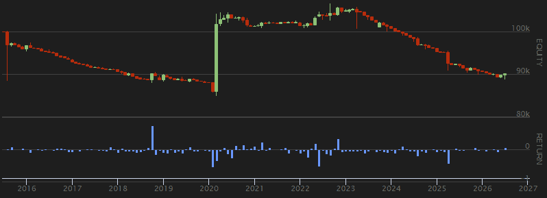
A more realistic alternative may be to submit the rebalancing order 10 minutes before the market close and execute it at the prevailing market price. This avoids relying on the exact closing price, but it also does not necessarily represent the optimal execution. The market can still move substantially during the final minutes of trading, particularly for highly leveraged ETFs such as TQQQ and SQQQ.

Table 3: Returns of the daily rebalanced strategy with order 10 minutes before close, executed EOD.

Strategy	Return (total)	Return (yearly)	Volatility (yearly)	Sharpe
Daily rebalance EOD, order 10 minutes before close	-10.34%	-0.98%	3.9%	-0.25

Rebalancing frequency

After establishing the baseline results, we turn to the frequency of rebalancing. The simplest approach is to rebalance the portfolio every trading day. This keeps the two short positions close to their intended 50/50 allocation, but requires frequent transactions. An alternative is to rebalance once per week. While this reduces the number of transactions, it allows the relative weights of TQQQ and SQQQ to drift between rebalancing dates.

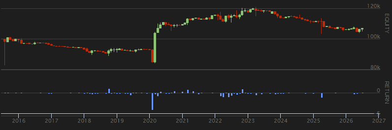
The weekly strategy introduces an additional issue: the choice of the particular day on which the rebalance is performed. We therefore evaluate the different possible weekly rebalancing days separately.

Table 4: Returns of the strategies rebalanced every 5th day with order 10 minutes before close, executed EOD, based on start day.

Strategy	Return (total)	Return (yearly)	Volatility (yearly)	Sharpe
Day 1 start	7.58%	0.66%	6%	0.11
Day 2 start	21.05%	1.74%	7.1%	0.25
Day 3 start	36.77%	2.87%	5.8%	0.49
Day 4 start	10.92%	0.94%	5.7%	0.16
Day 4 start	8.14%	0.71%	6%	0.12

This comparison is important because the strategy’s returns are not evenly distributed over time. If a substantial proportion of the total return is generated during a small number of high-volatility episodes, changing the rebalancing day can determine whether the portfolio is rebalanced before or after a particularly important market movement. And that is exactly what happend. By choosing specific start day of the strategy implementation, we can achieve vastly different results.

Introducing tranche-based rebalancing

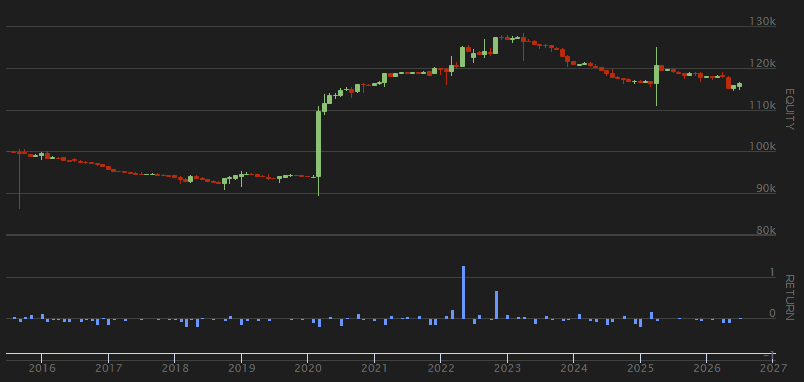
The sensitivity of weekly rebalancing to the selected day motivates an alternative implementation in which the required adjustment is distributed across several trading days. For a five-day rebalancing horizon, instead of performing the entire rebalance at once, we execute 20% of the required portfolio adjustment each day. This effectively replaces a single weekly execution with five smaller tranches.

Table 5: Returns of the strategy rebalanced in 5-day cycles with daily 20% tranches rebalances, orders 10 minutes before close, executed EOD.

Strategy	Return (total)	Return (yearly)	Volatility (yearly)	Sharpe
5D tranche strategy	15.6%	1.32%	4.7%	0.28

The five-day tranche-based strategy can be naturally generalized to an (N)-day rebalancing cycle. Instead of executing the entire portfolio adjustment at once, the required rebalancing is divided into (N) equal tranches, with one tranche executed on each trading day. Thus, the five-day version can be viewed as a special case of a more general (N)-day tranche-based strategy.

To examine whether a longer execution horizon provides a more robust implementation, we consider two additional specifications: 10-day and 20-day tranche-based rebalancing. In each case, the portfolio adjustment is distributed evenly across the corresponding number of trading days.

Table 6: Returns of the strategies rebalanced in 10/20-day cycles with daily 10%/5% tranches rebalances, orders 10 minutes before close, executed EOD.

Strategy	Return (total)	Return (yearly)	Volatility (yearly)	Sharpe
10D tranche strategy	27.15%	2.19%	6.5%	0.34
20D tranche strategy	25.66%	2.09%	9%	0.23

The results become relatively similar as the length of the tranche-based rebalancing horizon increases. The 10-, and 20-day versions exhibit broadly comparable performance, suggesting that the exact choice of the tranche horizon is less important than the use of tranche-based rebalancing itself.

At the same time, the results reveal a common feature across all three specifications. Even in these more robust implementations, the strategy does not generate its returns continuously over the sample period. Instead, the majority of the cumulative return is concentrated in a relatively small number of periods associated with macroeconomic events and market disruptions that led to elevated volatility. These include episodes such as the COVID-19 crisis, the outbreak of the war in Ukraine, and Liberation Day. Thus, although tranche-based rebalancing makes the results less sensitive to the precise timing of individual rebalancing transactions, it does not fundamentally change the source of the strategy’s profitability.

Conclusion

In this paper, we examined a strategy that exploits the volatility decay of leveraged ETFs by simultaneously shorting TQQQ and SQQQ in equal proportions. The opposite exposures of the two ETFs make the resulting portfolio approximately directionally neutral, allowing the strategy to target volatility decay rather than the direction of the Nasdaq-100.

The results show an important difference between the theoretical attractiveness of the strategy and its performance under more realistic assumptions. While the benchmark without borrowing costs produces nearly 4% annual return, incorporating borrowing costs substantially changes the picture. The return generated by volatility decay is not sufficient to provide a persistent source of net profitability across ordinary market conditions.

We also find that the implementation of the rebalancing rule matters. The results of weekly rebalancing can vary considerably depending on the selected rebalancing day, while the comparison of EOD and pre-close execution highlights the sensitivity to the precise execution convention. Tranche-based rebalancing provides a more robust alternative. The 10-, and 20-day versions produce relatively similar results, suggesting that the exact length of the tranche horizon is less important once the rebalancing is distributed across multiple days.

Despite this increased robustness, the underlying pattern remains unchanged. The strategy generates most of its returns during a small number of periods characterized by exceptionally high market volatility, typically associated with major macroeconomic or geopolitical events. Outside these episodes, the strategy is largely neutral after borrowing costs.

Overall, our results suggest that volatility decay in leveraged ETFs can indeed be exploited through a market-neutral short TQQQ-SQQQ portfolio, but the resulting return should not be interpreted as a stable arbitrage premium. Once borrowing costs and implementation details are taken into account, the profitability of the strategy becomes highly conditional on the occurrence of periods of elevated volatility. This highlights the importance of incorporating realistic trading costs and execution assumptions when evaluating strategies based on leveraged-ETF decay.

Authors:

David Belobrad, Junior Quant Analyst, Quantpedia

Filip Kalus, QuantConnect Code Builder, Quantpedia

---

Are you looking for more strategies to read about? Sign up for our newsletter or visit our Blog or Screener.

Do you want to learn more about Quantpedia Premium service? Check how Quantpedia works, our mission and Premium pricing offer.

Do you want to learn more about Quantpedia Pro service? Check its description, watch videos, review reporting capabilities and visit our pricing offer.

Do you want algorithmic access to the full Quantpedia database via the API? Subscribe to Quantpedia Pro, ask for an API key, and explore the in/out-of-sample statistics, source academic papers, and code snippets — ideal for quantitative research, systematic trading workflows, and AI model training.

Are you looking for historical data or backtesting platforms? Check our list of Algo Trading Discounts.

---

Or follow us on:

Facebook Group, Facebook Page, Telegram, Twitter, Linkedin, Medium or Youtube

References:

1. https://quantpedia.com/strategies/arbitraging-levered-etfs ↩︎
2. https://papers.ssrn.com/sol3/papers.cfm?abstract\_id=4146736 ↩︎
3. https://quantpedia.com/strategies/volatility-decay-and-arbitrage-in-leveraged-etfs ↩︎
4. https://papers.ssrn.com/sol3/papers.cfm?abstract\_id=5421274 ↩︎
5. https://valuelytica.substack.com/p/vdc-qqq ↩︎

Share onLinkedInTwitterFacebookRefer to a friend